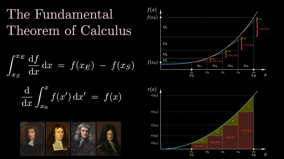
The Fundamental Theorem of Calculus

In this and a few subsequent posts I will try to cover some of the basics of one of the most important branches of Mathematics: Calculus. It focuses on a basic/introductory level, but not all of basic calculus will be covered, as there is already the excellent and very popular series of YouTube videos by Grant Sanderson, a.k.a. "3Blue1Brown", which I recommend as a supplement. The goal is to provide an intuitive understanding of the concepts involved.

A bit of history

We begin with a bit of history. The invention of Calculus in the 17^th century was arguably the single most important development in Mathematics since the time of Archimedes (3^rd century BC). It was invented in order to solve pressing scientific problems of that era, which could not be solved by the existing mathematical tools of geometry and algebra. Calculus catalysed scientific progress and enabled all sorts of developments in science and engineering, playing a crucial role in shaping the modern world.

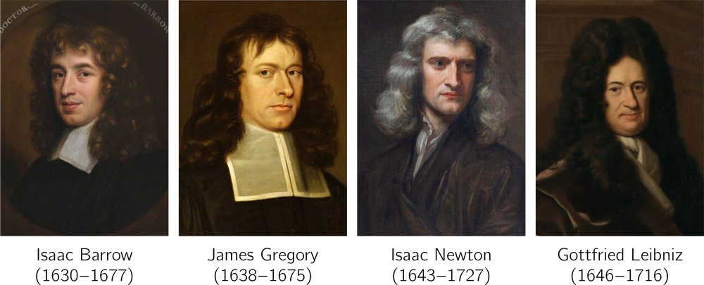
The invention of calculus is commonly attributed to Isaac Newton and Gottfried Wilhelm Leibniz. Newton developed his theory first, but Leibniz was the first to publish his own work on calculus. This led to a bitter controversy over who was the first to discover calculus, with Newton and his camp accusing Leibniz of plagiarising. The modern consensus is that the two men developed their ideas independently, but this has not been proved beyond doubt. The history of the controversy is intriguing, but unfortunately it is also beyond the scope of the present post. A couple of papers that may satisfy the reader who is curious to learn more about it are Hall (2004)^[1] and Blank (2009)^[2]. I cannot resist, however, the temptation to include, as a teaser, the following quote from the latter paper:

"Historians and sociologists of science have long been fascinated with multiple discoveries – clusters of similar or identical scientific advances that occur in close proximity if not simultaneously. Such discoveries are even more noteworthy when they exemplify the phenomenon of convergence – the intersection of research trajectories that have different initial directions. Throw in a priority dispute, charges of plagiarism, and two men of genius, one vain, boastful, and unyielding, the other prickly, neurotic, and unyielding, one a master of intrigue, the other a human pit bull, each clamoring for bragging rights to so vital an advance as calculus, and the result is a perfect storm. The entire affair – the most notorious scientific dispute in history – has been exhaustively scrutinized by scholars".
Blank (2009)^[2:1]

---

1. Hall, A. R. (2004). Newton versus Leibniz: from geometry to metaphysics. In: Cohen, I. B. & Smith, G. E. (Ed.), The Cambridge Companion to Newton, Cambridge University Press. ↩︎

2. Blank, B. E. (2009). The Calculus Wars reviewed by Brian E. Blank, Notices of the American Mathematical Society 56 : 602-610. ↩︎ ↩︎

0:00

/0:12

1×

The above quote highlights that intellectual brilliance does not guarantee moral integrity. That said, I admit to being somewhat sympathetic toward figures like Newton and Leibniz because their extraordinary intellectual gifts must have placed immense pressure on their egos, and in such circumstances, maintaining humility is no easy feat. But the quote also points out something else of interest: that the discovery/invention of calculus seems to have occurred at a point of convergence of research trajectories. If we are to be fair, Newton and Leibniz should not be given all the credit for the discovery. Newton himself acknowledged, "If I have seen further it is by standing on the shoulders of Giants". And indeed the contributions of many mathematicians across the centuries accumulated until the breakthrough was made. Among them are Antiphon and Bryson of Heraclea (5^th century BC), Eudoxus (4^th century BC), Archimedes (3^rd century BC), Nicole Oresme and the Oxford Calculators (14^th c.), and, in the 17^th century, Johannes Kepler, Bonaventura Cavalieri, René Descartes, Pierre de Fermat, John Wallis, James Gregory, and Isaac Barrow – culminating in the work of Newton and Leibniz.

We notice that the foundations were laid in antiquity, then there was a large gap, followed by a resurgence of interest leading up to a heavy clustering of developments in the 17^th century. Thus it is apparent that is not just by the fortune of having such brilliant mathematicians as Newton and Leibniz that calculus came to be, but the time was ripe.

Calculus is the branch of mathematics concerned with derivatives, commonly understood as the slopes of curves, and integrals, which are often interpreted as the areas bounded by curves. At the heart of calculus lies the fundamental theorem of calculus, which links the two together, or, to put it more meaningfully, links the rate of change of something to its total accumulated change. This fundamental theorem is the topic of this post. As it happens, it was first proved independently by James Gregory and Isaac Barrow shortly before Newton and Leibniz made their famous advancements. Isaac Barrow, a priest with an interesting life that included travelling to the Ottoman empire and encountering pirates, was in fact Newton's teacher and his predecessor as Lucasian Professor of Mathematics. This connection underscores the point that attributing the invention of calculus to Newton and Leibniz alone is an oversimplification. Barrow demonstrated how to compute the area under a curve by constructing another curve whose slope corresponds to the height of the original curve − see Bressoud (2011)^[1] for details. This is a particularisation of the fundamental theorem of calculus to areas and slopes. Newton and Leibniz, however, grasped the generality and power of the method and developed calculus into a comprehensive and widely applicable mathematical framework.

---

1. Bressoud, D. M. (2011). Historical Reflections on Teaching the Fundamental Theorem of Integral Calculus, The American Mathematical Monthly 118 : 99-115. ↩︎

Providing a detailed historical account is beyond the scope of this post. To learn more about the history of calculus you can check the aforementioned bibliography, and also the very nice series of videos in Tarek Said's YouTube channel. We will now jump to the modern concepts and explain the core idea of the theorem.

---

In a nutshell

So, what is the fundamental theorem of calculus all about? In a nutshell, as already mentioned, it describes the relationship between the rate of change of some quantity and the total accumulated change of that quantity. The standard example, and a primary application in the historical development of calculus, is the relationship between a moving object's velocity and the total distance it has travelled. The object's velocity is the rate of change, or derivative, of the distance travelled with respect to time; and conversely, the total distance travelled by the object is the accumulated effect, or integral, of the velocity over the whole time interval that the motion took place. Differentiation is the operation that gives us the velocity if we know the time history of the distance travelled; and integration is the operation that gives us the distance travelled if we know the time history of the velocity. Differentiation and integration are, therefore, inverse operations.

0:00

/0:03

1×

Let us break it down. Let us begin with the derivative, or rate of change. Immediately, we notice that the rate of change of a quantity (of distance, in this example) is only meaningful with respect to another quantity (time, in this example). Usually, when we talk of rate of change, we implicitly understand it to be with respect to time – how quickly something changes as time passes. But it is useful to generalise this idea to all kinds of dependencies between quantities; for example:

• The rate of change of atmospheric pressure with respect to the altitude (units: Pa/km).
• The rate of change of the area of the square with respect to the length of its side (units: m²/m).
• The rate of change of the length of a spring with respect to the applied force (units: m/N).
• The rate of change of the total electricity cost with respect to the amount of energy consumed (units: €/kWh).

For the rate of change to be meaningful, one quantity must be connected to another, so that a change in one implies a change in the other. In mathematical terminology, we say that one quantity is a function of the other. It is convenient to regard one of the quantities as free for us to change however we please, which we call the independent variable; in the previous examples, it is time, the altitude, the length of the square, the applied force, and the energy consumed (the quantities printed in bold). Then the other quantity does not change freely, but its own change is determined by the corresponding change of the independent variable. We thus call it the dependent variable (in the examples: distance or velocity, atmospheric pressure, area of the square, length of the spring, electricity cost – the quantities highlighted). It is then meaningful to ask the question of how a change in the dependent variable depends on a change in the independent variable.

The rate of change of the dependent quantity with respect to the independent one is expressed mathematically as the ratio between corresponding changes. Thus, the physical units of the rate of change are equal to the ratio of units of the dependent quantity to those of the independent quantity. In the examples, these are metres per second or metres per second squared, pascals per kilometre, square metres per metre, metres per newton, euros (or dollars) per kilowatt-hour.

For instance, in the last example, if the rate is 0.3 €/kWh, this means that for each kWh of energy that we consume we have to pay 0.3 €. Therefore, if we consume 1 kWh we have to pay 0.3 €, if we consume 2 kWh we have to pay 0.6 €, if we consume 3 kWh we have to pay 0.9 €, etc. If we plot the dependent variable, i.e. the cost, versus the independent variable, i.e. the energy consumed, then we get a straight line.

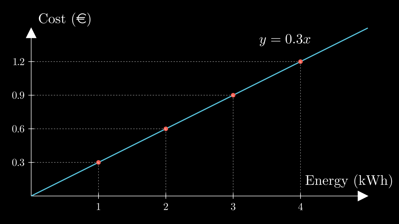
The slope of this line, defined as the ratio of a change in the dependent variable to the corresponding change in the independent variable, is constant, and equal to 0.3 €/kWh, so that choosing any amount of energy consumed and dividing the corresponding cost by that amount we always get the same result, the fixed rate. For example, for some of the points marked with red dots in the above plot, we have:

$$ \text{rate} \quad r \;=\; \frac{0.3\text{ €}}{1 \text{ kWh}} \;=\; \frac{0.6\text{ €}}{2 \text{ kWh}} \;=\; \frac{0.9\text{ €}}{3 \text{ kWh}} \;=\; 0.3\text{ € / kWh} $$

If we know this rate of change, then we can calculate the total accumulated cost by multiplying the rate by the total consumed energy:

$$ \text{cost} \;=\; \text{rate} \;\times\; \text{energy} $$

For example,

• Cost of 1 kWh = rate × (1 kWh) = (0.3 €/kWh) × (1 kWh) = 0.3 €
• Cost of 2 kWh = rate × (2 kWh) = (0.3 €/kWh) × (2 kWh) = 0.6 €
• Cost of 3 kWh = rate × (3 kWh) = (0.3 €/kWh) × (3 kWh) = 0.9 €

and so on.

Similarly, consider the standard example of velocity as the rate of change of distance travelled: if we plot the distance travelled versus time for an object travelling at constant speed we will again get a straight line. The slope of this line is equal to a distance travelled divided by the corresponding elapsed time, which is of course the velocity (in metres per second, kilometres per hour, etc.).

0:00

/0:07

1×

Again, knowledge of this rate (the velocity) allows us to calculate the distance travelled during some amount of time, by multiplying the rate by the elapsed time. For example, for the case illustrated in the above plot where a car travels at a constant speed of 10 m/s, the distance travelled by the car during the first 3 seconds can be calculated as:

$$ s(t\!=\!3\,\text{s}) \;=\; (\text{velocity}) \times (\text{time}) \;=\; (10 \; \text{m/s}) \times (3 \; \text{s}) \;=\; 30 \; \text{m} $$

How about if we want to calculate the distance travelled between t = 2 s and t = 6 s? Knowledge of the constant velocity makes this easy too:

$$ \begin{align*} s(t\!=\!6\,\text{s}) \;-\; s(t\!=\!2\,\text{s}) \;&=\; (\text{velocity}) \times (\text{time interval}) \\[0.2cm] \;&=\; (10 \; \text{m/s}) \times (6 - 2 \; \text{s}) \;=\; 40 \; \text{m} \end{align*} $$

And, more generally, the distance travelled between times t₁ and t₂ can be easily calculated as

$$ s(t_2) - s(t_1) \;=\; v \times (t_2 - t_1) $$

where v is the constant velocity.

In general, if we know the rate of change of one quantity with respect to another, and this rate is constant, then a change in the dependent quantity equals the product of the rate times the corresponding change in the independent quantity.

But what if the rate of change is not constant? What if a car moves at variable speed, for example? How is the rate of change defined in that case? Our cars have indicators that inform us of our current speed, in km/h – but what does it mean if, say, my car's speed indicator reads 50 km/h? Well, it does not literally mean that in the next hour I will travel 50 km, for my whole trip might last only 10 minutes, or during that hour I might travel more than 50 km if I am about to enter a highway and increase my speed. Rather, what it means is that if I fix my speed at its current value for a whole hour, then I will cover a distance of 50 km. But what is the current speed, or in other words the instantaneous rate of change of my position? "Rate of change" implies change, and for a change to occur, some time has to pass, but something being instantaneous implies that no time has passed. "Instantaneous rate of change" sounds like an oxymoron; and yet our intuition tells us that there is such a thing – at each given instant something appears to move at a certain speed which may increase or decrease over time. This is what our car's speedometer displays.

0:00

/0:07

1×

To arrive at a meaningful definition, we begin with the observation that usually if we plot a function, as we zoom in close to any specific value of the independent variable, the plot of the function looks more and more like a straight line. Therefore, if we zoom in close enough, then we can assume the function to be a straight line locally and calculate the rate of change in the usual way, as the ratio of a change in the dependent variable to the corresponding change in the independent variable. Note that both of these changes must be very small, because we have zoomed in quite a lot. More precisely, we define the rate of change as the limit of this ratio when the change in the independent variable tends to zero – of course, this implies that the change in the dependent variable also tends to zero, if our function is well-behaved.

0:00

/0:21

1×

Therefore, the local rate of change r(x) of the dependent variable f(x) with respect to x, at some given value of x, is equal to

$$ \begin{equation} \label{r=df/dx} r(x) \;=\; \frac{\mathrm{d}f}{\mathrm{d}x} \end{equation} $$

where dx is a small change of x and df is the associated change in f, as long as the change dx is small enough such that we are confined within a small neighbourhood around the point x where f(x) behaves linearly.

Having obtained the rate of change, or derivative, of f(x) with respect to x from eq. ($\ref{r=df/dx}$), we can now calculate any change of f due to some small change in x, as:

$$ \begin{equation} \label{df=rdx} \mathrm{d}f \;=\; r(x) \, \mathrm{d}x \end{equation} $$

Of course, one would be justified to protest that the reasoning here appears circular: equation ($\ref{df=rdx}$) uses r to find df, but r itself was obtained from df through equation ($\ref{r=df/dx}$)! Indeed, eq. ($\ref{df=rdx}$) is nothing but a reformulation of eq. ($\ref{r=df/dx}$); the two equations are equivalent. Their jobs seem to be inverses: while eq. ($\ref{r=df/dx}$) uses df to find r, eq. ($\ref{df=rdx}$) uses r to recover df. This is precisely why differentiation (an operation expressed by eq. ($\ref{r=df/dx}$)) is the inverse of integration (an operation at the heart of which lies eq. ($\ref{df=rdx}$)).

In practice, if f(x) is known analytically, we usually obtain the rate function from eq. ($\ref{r=df/dx}$) using well-known mathematical techniques of differentiation, which give us the ratio df/dx in the limit $\mathrm{d}x \rightarrow 0$. Otherwise, we can calculate r(x) approximately using a small enough value of dx in eq. ($\ref{r=df/dx}$). This may be necessary in practical applications where f(x) is not known analytically (i.e. we don't have a mathematical equation expressing explicitly how its value relates to the value of x), such as when a car's speedometer calculates the rate of change of distance travelled. Anyway, once we obtain the local rate r(x) from eq. ($\ref{r=df/dx}$), we can use it to calculate the change df of the dependent variable for any small-enough change dx of the independent variable using eq. ($\ref{df=rdx}$) (the dx used in eq. ($\ref{df=rdx}$) need not be the same as that used in eq. ($\ref{r=df/dx}$)) as long as dx is small enough such that we remain confined to a neighbourhood where f(x) varies linearly.

But suppose that the change in the independent variable, Δx = x_E − x_S, is not small. If we know the variable rate of change, r(x), of f(x) with respect to x, how can we use this knowledge to calculate the corresponding change Δf = f(x_E) − f(x_S)? For example, if I have recorded the readings of my car's speedometer throughout my trip, how can I use this information to calculate the total distance travelled? What we can do is illustrated in the figure below. We can split the large change Δx into very small incremental changes dx each of which is small enough such that f varies linearly across it, calculate the corresponding changes df from eq. ($\ref{df=rdx}$), and sum all of them, to obtain:

$$ \begin{equation} \label{FTC precursor} \Delta f \;=\; f(x_E) - f(x_S) \;=\; \sum_{x=x_S}^{x=x_E} \mathrm{d}f_i \;=\; \sum_{x=x_S}^{x=x_E} r(x_i) \, \mathrm{d}x_i \end{equation} $$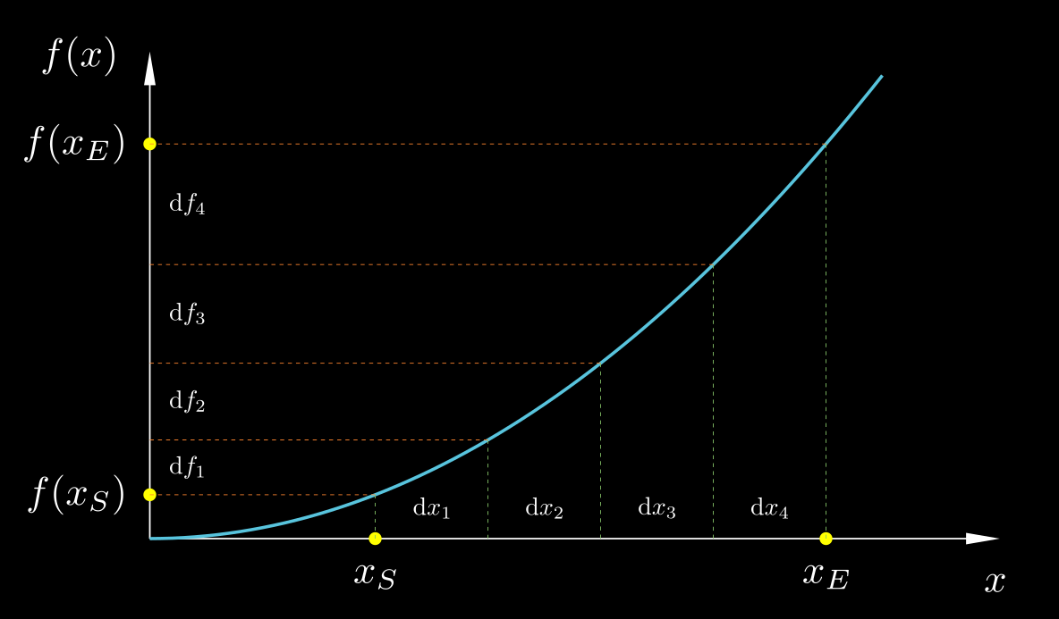

In order for this equality to hold, the x-changes, dx, must be extremely small, tending to zero; in this case, the sum is that of an infinite number of infinitesimal terms, and we call that an integral:

$$ \begin{equation} \label{FTC} f(x_E) - f(x_S) \;=\; \int_{x_S}^{x_E} \mathrm{d}f \;=\; \int_{x_S}^{x_E} r(x) \, \mathrm{d}x \;=\; \int_{x_S}^{x_E} \frac{\mathrm{d}f}{\mathrm{d}x} \, \mathrm{d}x \end{equation} $$

Does this equation look familiar? It is the fundamental theorem of calculus!

Let us use eq. ($\ref{FTC}$) to solve the following problem. Suppose a known function r(x), and suppose that we want to find the function f(x) whose derivative is r(x). In other words, we want to find f(x) such that r(x) = df/dx. Put yet differently, if r(x) is interpreted as a rate of change, whose rate of change is it?

We should first note that there are infinitely many such functions f(x), with any two of them differing by a constant. (Adding a constant to a function has no effect on its rate of change; it shifts the entire curve of the function up or down, but its slope remains unchanged). Therefore, to make f(x) specific, let us assume that we know its value f(x₀) at some given point x₀. Then, let us use x₀ as the starting point x_S in eq. ($\ref{FTC}$), and let the ending point x_E be any random point x. Having reserved the name x for the end point of the independent variable, we must use a different name for the value of the independent variable as it varies between x₀ and x during the process of integration; we will use the name x'. That is, since we decided to replace the symbol x_E with x in eq. ($\ref{FTC}$), but that equation already employed the symbol x, we must change that latter x with another symbol, and we choose x'. Of course, both x and x' refer to the independent variable, but they refer to different values of it: x refers to the upper limit of integration, while x' varies between the lower and upper limits as we integrate. With all these considerations, eq. ($\ref{FTC}$) becomes:

$$ \begin{equation} \label{FTC indefinite} f(x) - f(x_0) \;=\; \int_{x_0}^x r(x') \, \mathrm{d}x' \quad\Rightarrow\quad f(x) \;=\; f(x_0) \;+\; \int_{x_0}^x r(x') \, \mathrm{d}x' \end{equation} $$

Equation ($\ref{FTC indefinite}$) tells us how to find the function f(x) whose rate of change with respect to x is r(x), and whose value at point x₀ is f(x₀).

So, there you go. That's the fundamental theorem of calculus. But, you may ask in surprise, is that all? Where is the talk about areas under curves – the common interpretation of integrals? In my opinion, the interpretation of the integral as an area is a secondary one. The main meaning of the integral is what was just presented: the integrated function should be viewed as a rate of change, and the integral as the total change. This concept has far greater generality.

For example, in vector calculus (if you are not familiar with vector calculus, just ignore what I'm about to say – perhaps I'll devote another post to it) we can straightforwardly apply this fundamental theorem to evaluate the integral along a curve. If 1 and 2 are two points on some curve, and ϕ₁ and ϕ₂ are the corresponding values of some function ϕ at these points, and if we break the curve up into infinitesimal vectors $\mathrm{d}\vec{s}$, then from the definition of $\nabla \phi$ the following should make sense:

$$ \int_1^2 \nabla \phi \cdot \mathrm{d}\vec{s} \;=\; \int_1^2 \mathrm{d}\phi \;=\; \phi_2 - \phi_1 $$

(Again, if the above equation does not make sense to you, don't worry. Just ignore this example).

Hopefully, the explanation leading up to equations ($\ref{FTC}$) and ($\ref{FTC indefinite}$) should make the fundamental theorem of calculus look straightforwardly intuitive. If an intuitive grasp of the theorem is all you want, you can skip the rest of this essay. But if you are interested in delving a bit deeper, including about the nuances of evaluating derivatives and integrals, and the interpretation of the integral as the area under a curve, keep reading.

Derivatives

Let us begin with a deeper look into differentiation. Consider a function f(x). Consider the change in its value, f(x₂) − f(x₁), across the interval [x₁, x₂]. Changing the value of the independent variable from x₁ to x₂ causes the value of the function to change from f(x₁) to f(x₂). So, we could say that the average rate of change of f with respect to x in the interval [x₁, x₂] is equal to the ratio:

$$ \begin{equation} \label{r_avg} \bar{r}_{[x_1,x_2]} \;=\; \frac{f(x_2) - f(x_1)}{x_2 - x_1} \end{equation} $$

Now, suppose we want to determine the instantaneous rate of change at some point x. By "instantaneous" we mean that it does not refer to an interval but just to the single point x. One idea, then, would be to use eq. ($\ref{r_avg}$) and shrink the interval [x₁, x₂] down to the single point x, by making both of its endpoints equal to x. Unfortunately, this doesn't work, as setting x₁ = x₂ = x in eq. ($\ref{r_avg}$) makes both the numerator and the denominator of the fraction equal to zero. And it makes sense that this would fail, because a "rate of change" makes sense only if there is change, and if x₁ = x₂ then there is no change whatsoever. But we can take x₂ to be as close as we wish to x₁ without being equal to it. This is where the concept of limit comes in. If we imagine x₂ coming closer and closer to x₁, so that the distance between them goes towards zero, will the value of the above fraction tend towards some specific value? In most cases that we will encounter the answer is yes. Let us illustrate this in the case of the function f(x) = x². Let us choose one endpoint of the interval to be the point x itself, x₁ = x, and the other endpoint to be a distance $\delta x$ away, $x_2 = x + \delta x$, and let us see what happens to the ratio ($\ref{r_avg}$) if we make $\delta x$ smaller and smaller:

$$ \begin{align} \nonumber \frac{f(x _2) - f(x_1)}{x_2 - x_1} \;&=\; \frac{f(x + \delta x) - f(x)}{\delta x} \\[0.2cm] \nonumber \;&=\; \frac{(x+\delta x)^2 \,-\, x^2}{\delta x} \\[0.2cm] \nonumber \;&=\; \frac{\cancel{x^2} \,+\, 2 x \delta x \,+\, (\delta x)^2 \;-\; \cancel{x^2}}{\delta x} \\[0.2cm] \label{dfdx x2 FD} \;&=\; 2x \;+\; \delta x \end{align} $$

As $\delta x \rightarrow 0$, this value tends to the value $2x$. So, the average rate of change of f(x) = x² in the region $[x, x+\delta x]$ as this region shrinks towards x itself tends to $2x$. This limit value of the rate of change of f(x) at the point x is called the derivative of f(x), and is denoted as df/dx. The notations df and dx here imply that these changes are infinitesimal, that they tend to zero. So, for example, if the distance travelled by an object is given by s(t) = t², where s is in meters and t in seconds, then its instantaneous velocity at t = 5 s is equal to ds/dt = 2t = 2×5 = 10 m/s.

0:00

/0:14

1×

Now, in the above derivation, to find the derivative at the point x, we selected the interval [x₁, x₂] such that x was its lower endpoint. But this is not obligatory; there are many other options, and all that is required is that the region [x₁, x₂] shrinks towards the single point x. To illustrate this, let us choose the region [x₁, x₂] such that x is its midpoint: $x_1 = x - \delta x$, $x_2 = x + \delta x$. Let us again calculate the average rate of change across this region from eq. ($\ref{r_avg}$), and see what happens to it as the size of the region tends to zero, i.e. as $\delta x \rightarrow 0$.

$$ \begin{align} \nonumber \frac{f(x_2) - f(x_1)}{x_2 - x_1} \;&=\; \frac{f(x + \delta x) - f(x - \delta x)}{2 \delta x} \\[0.2cm] \nonumber \;&=\; \frac{(x+\delta x)^2 \,-\, (x-\delta x)^2}{2 \delta x} \\[0.2cm] \nonumber \;&=\; \frac{x^2 + 2 x \delta x + (\delta x)^2 \;-\; x^2 + 2 x \delta x - (\delta x)^2}{2 \delta x} \\[0.2cm] \label{dfdx x2 CD} \;&=\; 2x \end{align} $$

Very conveniently, in this case the average rate of change is the same irrespective of the size of the region! Nothing happens to it as we shrink the size of the region to zero (see the video below). Therefore, the value $2x$ is also the limiting value as $\delta x \rightarrow 0$, i.e. it is equal to the instantaneous rate of change at x.

0:00

/0:13

1×

One may wonder if this is always the case: does the average rate of change over an entire region equal the instantaneous rate of change at the centre of that region? The answer is no. It so happens in the special case of the quadratic function f(x)=x², but it does not hold in general. For example, you can verify yourself that the two methods applied to the cubic function f(x) = x³ give:

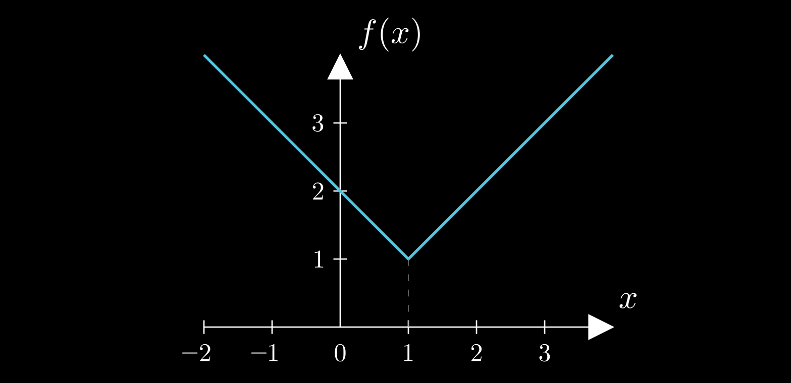
$$ \begin{equation} \label{x3 FD} \frac{f(x\!+\!\delta x)-f(x)}{\delta x} \;=\; \frac{(x\!+\!\delta x)^3 - x^3}{\delta x} \;=\; 3x^2 \;+\; 3 x\, \delta x \;+\; (\delta x)^2 \end{equation} $$ $$ \begin{equation} \label{x3 CD} \frac{f(x\!+\!\delta x)-f(x\!-\!\delta x)}{2\delta x} \;=\; \frac{(x\!+\!\delta x)^3 - (x\!-\!\delta x)^3}{2\delta x} \;=\; 3x^2 \;+\; (\delta x)^2 \end{equation} $$

Now it is in both cases that we need to shrink δx towards zero in order to obtain the instantaneous rate of change. But we notice again that, as for most functions that are of interest, how we construct the interval around x does not matter; in all cases, as we shrink that interval towards x itself we get the same limiting instantaneous rate of change. In the present case, we see that both formulae, ($\ref{x3 FD}$) and ($\ref{x3 CD}$), converge to the same value, 3x², as δx → 0, which we denote as df/dx. Not all functions are so well-behaved, though. Sometimes the limiting rate of change at x as the interval shrinks does depend on the type of interval chosen, such as, for example, when the function has a sharp corner at x (see the figure below); sometimes there isn't even a definite limiting value. In such cases we say that the function is not differentiable at x.

The left-hand sides of equations ($\ref{x3 FD}$) and ($\ref{x3 CD}$) can be viewed as approximations to the derivative df/dx. For obvious reasons, the expression ($\ref{x3 FD}$) is called a "forward difference" and the expression ($\ref{x3 CD}$) is called a "central difference". While both converge to the same limit value (the derivative), they do not do so at the same pace. By inspecting the right-hand sides of ($\ref{x3 FD}$) and ($\ref{x3 CD}$), we see that their respective errors are E_FD = 3x δx + (δx)² and E_CD = (δx)². The table below lists those errors at x = 2, for smaller and smaller values of δx. Each successive value of δx is half of the previous one. We observe that the central difference error diminishes more rapidly than the forward difference one – for the smallest δx listed, E_CD is nearly 100 times smaller than E_FD.

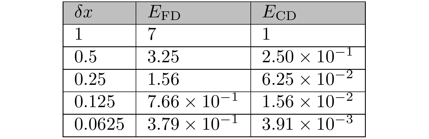
The central difference approximation ($\ref{x3 CD}$) is characterised as "second-order accurate" because its error, Ε_CD = (δx)², is proportional to the 2^nd power of δx. This has the consequence that each time we halve δx this error will become 4 times smaller (each of the two factors of (δx)² = δx×δx will be halved, hence their product will become 2×2 = 4 times smaller). This is precisely what we see in the last column of the above table. On the other hand, the forward difference approximation ($\ref{x3 FD}$) is characterised as "first-order accurate" which, as you can guess, means that its error, E_FD = 3x δx + (δx)², is proportional to the 1^st power of δx. Well, it is not exactly proportional to δx, because there is also the term (δx)²; but this term diminishes faster than its partner 3x δx, so that eventually at small enough δx it becomes negligible compared to it, and E_FD ≈ 3x δx. This is verified by the second column of the above table, which shows that halving δx causes E_FD to also nearly become half, so that E_FD and δx are roughly proportional. "First-order" and "second-order" refer to the asymptotic behaviour of the approximations, when δx → 0.

The forward and central difference approximations to the derivative exhibit first- and second-order accuracy, respectively, not only in this particular example but in general. Proving this requires knowledge of the theory of Taylor series, which may be the topic of another post, but let us just illustrate it with another example, that of the function sin(x). The derivative of sin(x) is cos(x) (see this video by 3Blue1Brown for a nice proof). The following video shows the sin(x) function together with its tangent at the point x₀ = π/3. The black and green dashed lines are approximations to this tangent, obtained by forward differences (which, in addition to the point x₀ also use the point x₁ = x₀ + δx, also marked in the plot), and central differences (which uses the points x₁ = x₀ + δx and x₂ = x₀ − δx, also marked on the plot), respectively. The video shows what happens as the approximation step δx is varied, but in general it is obvious that central differences provide much more accurate approximations to the slope of sin(x) than forward differences.

0:00

/0:08

1×

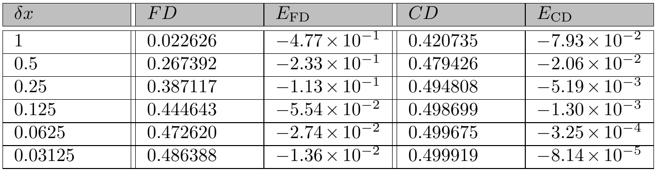
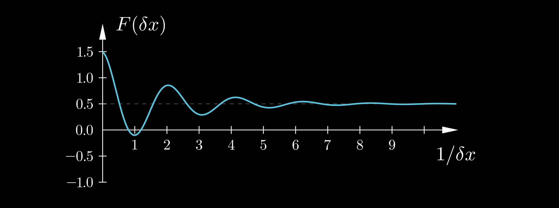
For a more quantitative assessment of the accuracy of the finite difference approximations, the following table presents their predictions of d(sin(x))/dx at x₀ = π/3, which equals cos(π/3) = 0.5, for various values of δx. As before, each successive value of δx is half of the previous one. The predictions of both forward and central differences converge towards the correct value 0.5 as δx tends to zero. However, again CD converges faster, with each successive halving of δx resulting in the E_FD and E_CD errors becoming roughly 2 and 4 times smaller, respectively. Therefore, again E_FD ~ δx while E_CD ~ δx² (the tilde ~ here meaning "is proportional to"). In other words, FD exhibits first-order convergence while CD exhibits second-order convergence, their expected behaviours.

Limits

As said, the above table suggests that both the FD and CD converge to the exact value of the derivative, 0.5, as δx is made smaller. How do we know that? Well, we see the decimals of the finite differences, and they seem to be headed towards the value 0.5, which we know is the exact value because we are aware of the theoretical result that the derivative of sin(x) is cos(x), and the value of cos(x) at x = π/3 is 0.5. Both the FD and the CD appear to approach the value of 0.5 from below, i.e. they give a slope less than 0.5 but their prediction increases towards 0.5 as δx is reduced (we can see this also in the above video, where the slopes of the FD and CD lines increase towards the slope of the tangent as δx is reduced).

We say that 0.5 is the limit of the FD and CD as δx → 0. How can we formally define this limit? Can we simply say that it is the number to which the FD or CD come closer and closer as δx is reduced? Unfortunately this simplistic "definition" is not precise enough, as with each subdivision of δx, FD and CD come closer and closer also to 0.51, to 0.55, to 1, and indeed to any number R > 0.5. What makes the value r = 0.5 special compared to all these other values is that the FD and CD can get arbitrarily close to it, whereas they cannot do so for any of the other values R > 0.5. For example, FD and CD cannot approach the value R = 0.6 beyond a margin of 0.6 − 0.5 = 0.1.

So, could this be the definition we are looking for? That "the limit is the value that the finite differences can get arbitrarily close to"? As it turns out, there is something missing from this definition as well. There are plenty of values smaller than 0.5 that the finite differences get arbitrarily close to; in fact they become equal to them for some δx.

How about, "the limit is the value that the finite differences can get arbitrarily close to, but never reach". This would work in our particular example, as the only value for which this holds is 0.5. But in general, it doesn't always work. To illustrate the problem, suppose that CD's were not strictly increasing as δx is reduced, but converged to 0.5 with damped oscillations. In that case, the precise value 0.5 would be reached every now and then, in fact infinitely many times. Our definition would therefore erroneously reject the value 0.5 as the limit.

So, it seems that coming up with a precise expression of what the limit is, is not so easy. There are two necessary ingredients: One is arbitrary closeness, as we noted. The other is that a limit (and also the derivative, which is a specific kind of limit), though defined at a single point (for example as δx approaches the specific value of zero in our case), actually captures how the function behaves throughout an entire neighbourhood around that point. So, arbitrary closeness to some value at a single point is irrelevant, but what matters is arbitrary closeness over an entire neighbourhood, however small, around our point.

For a general function f(x), mathematicians have come up with the following definition which expresses these ideas. The limit of f(x) as x approaches the value p is equal to L,

$$ \lim_{x \rightarrow p} f(x) = L $$

if for every real ε > 0 there exist real δ > 0 such that |f(x) − L| < ε for all real x that satisfy 0 < |x − p| < δ.

Now, this may seem complicated at first glance, but "for every real ε > 0" establishes arbitrary closeness (since we can make the closeness ε as small as we wish), while "there exist real δ > 0" ensures that this closeness applies to an entire neighbourhood of points around p. (Of course, if there is such a δ then any other δ' < δ will also do). Note that the point p itself is excluded from the neighbourhood. The value f(p), if it is defined at all, contributes nothing to the limit.

That was about a general function. Now let us consider the particular functions of interest, namely FD and CD, given by the left-most expressions of eqs. ($\ref{x3 FD}$) and ($\ref{x3 CD}$). While those definitions contain the symbol x, that symbol denotes some fixed point and the independent variable is actually δx. So, in the above definition of a limit we must substitute x with δx. Now, since we are interested in what happens when δx → 0, we must also substitute p with 0. Therefore, if δf/δx stands for any of FD or CD, while df/dx is the exact derivative, then the finite differences will converge to the derivative if:

For every real ε > 0 there exist real δ > 0 such that |δf/δx − df/dx| < ε for all real δx that satisfy 0 < |δx| < δ.

To check whether FD and CD converge to df/dx as δx → 0 we therefore need to check that |δf/δx − df/dx|, i.e. the errors E_FD and E_CD listed in the respective columns of table 2, tend to zero as δx becomes smaller and smaller. Indeed, this is the case. If the behaviour of FD is such that its error is proportional to δx, and the behaviour of CD is such that its error is proportional to (δx)², which is what the numerical results suggest, then the above definition is satisfied and indeed the value 0.5 is the limit of both FD and CD.

Before turning to integrals, let us revisit the idea of the derivative as the "instantaneous" rate of change – a phrase that may sound like an oxymoron at first, as we previously noted. What is important to realise now is that although the derivative is defined at individual points, its value at a point encodes information about how the differentiated function behaves in an entire neighbourhood around that point – this is a direct consequence of the derivative being defined as a limit. The derivative, therefore, tells us something about what happens at neighbouring points as well. In particular, knowledge of the value of the derivative of a function at some point allows us to estimate the value of that function at neighbouring points through δf ≈ (df/dx)δx, which is the basis of the fundamental theorem of calculus.

Integrals

So, let us consider the reverse problem now. Suppose that we know the rate of change (for example, a vehicle's speed as a function of time) and we want to calculate the overall change (the distance travelled, in this example). To make things more precise, suppose that the function f(x) is unknown, but its rate of change r(x) = df/dx is known. We want to calculate the total change of the value of f(x) between the points x = x_S and x = x_E. We have already sketched the procedure that is to be followed: we use a divide-and-conquer strategy whereby we split the range [x_S, x_E] into a large number of small intervals of size δx each; we calculate the change δf in the value of f across each such interval from eq. ($\ref{df=rdx}$); and we add together all the incremental changes δf of the function value to get the total change according to eq. ($\ref{FTC precursor}$). Of course, for any non-zero value of δx, our calculation will contain an error; but, intuitively, we can assume that by driving δx towards zero the accuracy will improve, and in the limit δx → 0 we will get the exact result. Hence, we arrive at eq. ($\ref{FTC}$), which is the fundamental theorem of calculus.

All this sounds reasonable on first impression. However, the ancient Greek philosopher Zeno of Elea (a Greek colony in southern Italy) would protest strongly. Zeno gained notoriety for his paradoxes, which he devised to challenge the common-sense notions of motion and plurality. Concerning motion, he considered time as a series of discrete instants, so that each object as it is within the present instant of time is motionless (this is his "arrow paradox"). Hence he considered motion to be impossible and he would certainly have rejected the associated idea of a derivative or instantaneous rate of motion. However, he would undoubtedly also object to the notion of an integral. We can infer this from a couple of his paradoxes.

In one such paradox, sometimes called "the antinomy of large and small", Zeno argues that if an object has any non-zero size, then it must be infinitely large. His reasoning is roughly this: anything extended in space must consist of parts, each of which is itself extended. But if each part can again be divided into smaller extended parts, and so on without end, then the object must have an infinite number of spatial parts. And since the size of the whole is the sum of the sizes of its parts, Zeno concludes that this sum must be infinite – and thus, the original object must be infinitely large. In modern terms, he is implicitly rejecting the idea that an infinite sum of infinitesimal quantities can yield a finite result – precisely the principle that underlies the integral. He believes that adding together infinitely many things gives an infinite result.

The other relevant paradox is Zeno's most famous: Achilles and the tortoise. In this scenario, Achilles, a swift runner, races a tortoise that is given a head start. Zeno argues that Achilles can never overtake the tortoise. His reasoning is this: by the time Achilles reaches the tortoise’s starting position, the tortoise will have advanced to a new point. When Achilles reaches that new point, the tortoise will have moved again, and so on. This process repeats endlessly. Each step Achilles takes closes the gap, but also reveals a new, smaller gap to close. In effect, Zeno argues, Achilles must complete an infinite sequence of increasingly smaller tasks, each consisting of reaching the tortoise’s most recent position. Thus, Zeno concludes, Achilles can never overtake the tortoise, even though he runs faster.

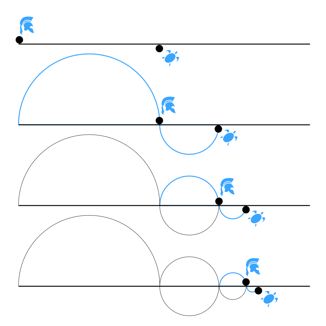
In both of these paradoxes, the surprising conclusion arises from Zeno’s assumption that an infinite sum must yield an infinite result. He reasons that if an object has infinitely many parts, it must be infinite in size. Likewise, in the case of Achilles and the tortoise, he assumes that the total distance Achilles must cover – the sum of infinitely many smaller intervals – is itself infinite. And because each distance takes some non-zero time to traverse, Zeno concludes that the sum of all these infinitely many time intervals must also be infinite. Hence, Achilles can never catch up to the tortoise.

Of course, it is not hard to see where Zeno's reasoning breaks down. When a volume is divided into smaller and smaller parts, the total volume remains constant because the size of each part decreases in proportion to their growing number. In the case of Achilles and the tortoise, knowing their respective speeds allows us to calculate exactly where Achilles will overtake the tortoise. The infinitely many, ever-shrinking distances that Achilles covers – each corresponding to a step in Zeno’s construction – add up not to infinity, but to a finite sum: the total distance to the meeting point. Still, Zeno’s paradoxes remind us to be cautious: when dealing with infinite processes, we must verify that the integral (or infinite sum) truly yields a finite result.

0:00

/0:27

1×

Let us, therefore, revisit our derivation of the fundamental theorem of calculus, and examine it more critically. Knowing the rate of change df/dx of the function f(x), we want to calculate the total change of the value of f(x) between the points x = x_S and x = x_E. Let us break the range [x_S, x_E] into N intervals [x_i, x_i+1] by introducing the intermediate points x_i, i = 1, 2, …, N+1, with x₁ = x_S and x_N+1 = x_E. We estimate the change in the value of f across each interval as:

$$ \begin{equation} \label{df=dfdx.dx} \delta f_i \;\approx\; \left. \frac{\mathrm{d}f}{\mathrm{d}x} \right|_{x_i^*} \! \delta x_i \end{equation} $$

where:

$ \delta f_i \;=\; f(x_{i+1}) - f(x_i) $

$ \delta x_i \;=\; x_{i+1} - x_i $

$\left. \dfrac{\mathrm{d}f}{\mathrm{d}x} \right|_{x_i^*}$ is the derivative evaluated at some point ${x_i^*} \in [x_i, x_{i+1}]$.

The equation ($\ref{df=dfdx.dx}$) is approximate, i.e. it involves some error for any non-zero δx_i; but according to our previous theory we would expect this error to diminish as δx_i → 0. The exact relative location of the point $x_i^*$ where the derivative is evaluated within [x_i, x_i+1] has an effect on the rate at which relation ($\ref{df=dfdx.dx}$) becomes more accurate as δx_i → 0, but no matter where within that interval $x_i^*$ is located, the relation ($\ref{df=dfdx.dx}$) will tend to become exact as δx_i → 0. Perhaps we can see this more easily by rearranging relation (11) as:

$$ \begin{equation} \label{dfdx fin.dif} \left. \frac{\mathrm{d}f}{\mathrm{d}x} \right|_{x_i^*} \;\approx\; \frac{\delta f_i}{\delta x_i} \end{equation} $$

It is not hard to recognise that if ${x_i^*=x_i}$ then ($\ref{dfdx fin.dif}$) expresses the forward difference approximation of the derivative at ${x_i^*}$ (the left-most expression in eq. ($\ref{x3 FD}$)) while if ${x_i^* = (x_i \!+\! x_{i+1})/2}$ (i.e. ${x_i^*}$ is the midpoint of the interval [x_i, x_i+1]) then ($\ref{dfdx fin.dif}$) expresses the central difference approximation of the derivative at ${x_i^*}$ (the left-most expression in eq. ($\ref{x3 CD}$)). In any case, an error will be involved (a smaller error if ${x_i^* = (x_i \!+\! x_{i+1})/2}$, a larger error if ${x_i^*=x_i}$, etc.), so we can express relation ($\ref{df=dfdx.dx}$) as an equality thus:

$$ \begin{equation} \label{df=dfdx.dx+e} \delta f_i \;=\; \left. \frac{\mathrm{d}f}{\mathrm{d}x} \right|_{x_i^*} \! \delta x_i \;+\; \epsilon_i \end{equation} $$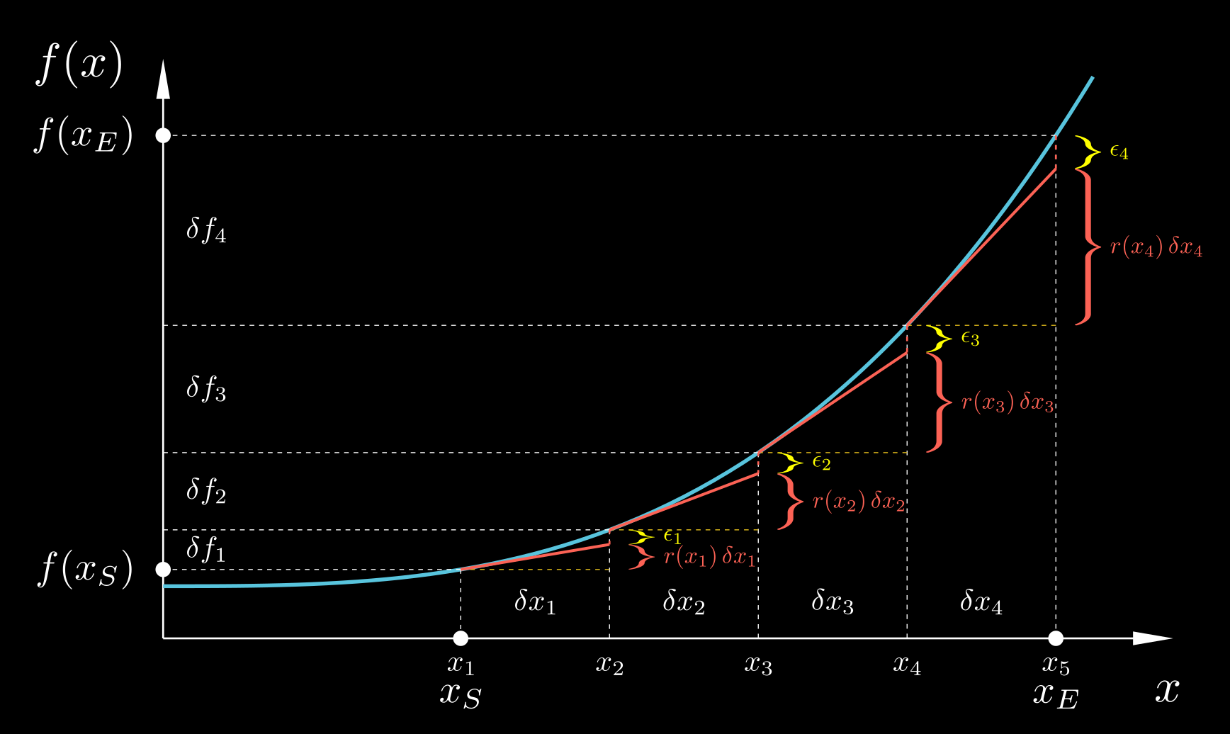

Then, to calculate the total change in the value of f(x) from x = x_S to x = x_E we add all the δf_i, as per eq. ($\ref{FTC precursor}$):

$$ \begin{equation} \label{FTC precursor e} f(x_E) - f(x_S) \;=\; \sum_{i=1}^{N} \delta f_i \;=\; \sum_{i=1}^{N} \left. \frac{\mathrm{d}f}{\mathrm{d}x} \right|_{x_i^*} \! \delta x_i \;+\; \sum_{i=1}^{N} \epsilon_i \end{equation} $$

The total error of the calculation ($\ref{FTC precursor}$) is, therefore, the sum of the individual errors $\epsilon_i$. A basic premise of calculus is that by making the δx_i smaller and smaller, i.e. by subdividing the interval [x_S, x_E] into more and more subintervals, the error in the calculation ($\ref{FTC precursor e}$) will diminish towards zero, arriving at equation ($\ref{FTC}$).

Is that so? If we examine eq. ($\ref{df=dfdx.dx+e}$), we see that as δx_i → 0 both its left-hand side (if f(x) is continuous) and the first term on its right-hand side tend to zero. Therefore, the error ϵ_i will also tend to zero. A naive thought, therefore, would be to conclude from this that Σϵ_i in ($\ref{FTC precursor e}$) will automatically also tend to zero as δx_i → 0 by virtue of the diminution of the individual errors being summed. But here is where Zeno would protest: he would claim that, on the contrary, as N → ∞ the total error in ($\ref{FTC precursor e}$) tends to become the sum of infinitely many individual errors, hence it becomes itself infinite in magnitude.

Who is right? Actually, both of these opposite naive views are flawed. We can use the same example as Zeno, of a finite volume being cut into infinitely many infinitesimal parts, to demonstrate that both arguments are wrong. As the volume is cut up into smaller and smaller pieces, the number of pieces tends to infinity, while their individual volumes tend to zero. But the total volume remains constant. Therefore, neither does the infinity of the number of parts mean that the sum of their volumes is infinite, nor does their infinitesimal size mean that this sum is zero. We must therefore examine the matter more meticulously.

That ϵ_i → 0 does not imply that Σϵ_i → 0 is also made apparent by the following observation. Let us substitute the derivative df/dx in eq. ($\ref{df=dfdx.dx+e}$) by an unrelated random function g(x). In the resulting equation,

$$ \begin{equation} \label{df=gdx+e} \delta f_i \;=\; g(x_i^*) \, \delta x_i \;+\; \epsilon_i \end{equation} $$

what happens if δx_i → 0? Well, δf_i = f(x_i+δx_i) − f(x_i) on the left-hand side tends to zero, but so does also the term $g(x_i^*) \delta x_i$ on the right-hand side. Hence, ϵ_i also tends to zero. Therefore, if it was true that ϵ_i → 0 implies that Σϵ_i → 0, then eq. ($\ref{FTC precursor e}$) would lead to

$$ \begin{equation} \label{FTC precursor wrong} f(x_E) - f(x_S) \;=\; \sum_{i=1}^{\infty} g(x_i^*) \, \delta x_i \end{equation} $$

or

$$ \begin{equation} \label{FTC wrong} f(x_E) - f(x_S) \;=\; \int_{x_S}^{x_E} g(x) \, \mathrm{d}x \end{equation} $$

for any two random and unrelated functions f(x) and g(x)! This is an absurd conclusion.

There has to be something special about r(x) = df/dx compared to all other random functions g(x) that makes the accumulated error Σϵ_i to decrease towards zero as we refine the δx_i intervals. To make it easier to see what this is, let us express the error in eq. ($\ref{df=dfdx.dx+e}$) in relative rather than absolute terms: $\epsilon_i = e_i \, \delta f_i$.

$$ \begin{equation} \label{df=dfdx.dx+e.df} \delta f_i \;=\; \left. \frac{\mathrm{d}f}{\mathrm{d}x} \right|_{x_i^*} \! \delta x_i \;+\; e_i \, \delta\! f_i \end{equation} $$

For the sake of simplicity, and without loss of generality, let us assume that all of the δf_i are equal: δf₁ = δf₂ = … = δf_N = δf. For monotonous continuous functions we can achieve this by suitably adjusting the size of each individual interval δx_i, using smaller δx where f(x) has larger slope and larger δx where f(x) has smaller slope. This is not something we can do if f(x) is not monotonous (i.e. not strictly increasing or strictly decreasing) but the point of the argument that we will make remains valid.

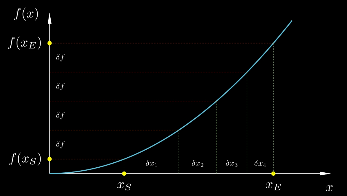
Let $\bar{e} = (\sum e_i)/N$ be the average of all the e_i's. Then, let us add all the δf_i's from eq. ($\ref{df=dfdx.dx+e.df}$), as in eq. ($\ref{FTC precursor e}$):

$$ \begin{align} \nonumber f(x_E) - f(x_S) \;=\; \sum_{i=1}^{N} \delta f \;&=\; \sum_{i=1}^{N} \left. \frac{\mathrm{d}f}{\mathrm{d}x} \right|_{x_i^*} \! \delta x_i \;+\; \left( \sum_{i=1}^{N} e_i \right) \delta f \\[0.2cm] \nonumber &=\; \sum_{i=1}^{N} \left. \frac{\mathrm{d}f}{\mathrm{d}x} \right|_{x_i^*} \! \delta x_i \;+\; \bar{e} N \delta f \\[0.2cm] \label{FTC precursor erel} &=\; \sum_{i=1}^{N} \left. \frac{\mathrm{d}f}{\mathrm{d}x} \right|_{x_i^*} \! \delta x_i \;+\; \bar{e} \left( f(x_E) - f(x_S) \right) \end{align} $$ $$ \begin{equation} \label{FTC precursor erel 2} \Rightarrow\; f(x_E) - f(x_S) \;=\; \frac{1}{1-\bar{e}} \; \sum_{i=1}^{N} \left. \frac{\mathrm{d}f}{\mathrm{d}x} \right|_{x_i^*} \! \delta x_i \end{equation}

where we have used that Σe_i = N$\bar{e}$ and that N δf = f(x_E) − f(x_S). We can see that the condition for eq. ($\ref{FTC precursor erel 2}$) to arrive at eq. ($\ref{FTC}$) in the limit of δx_i → 0 is that

$$ \begin{equation} \label{FTC condition} \lim_{\delta x \rightarrow 0} \bar{e} \;=\; 0 \end{equation} $$

Is this condition met? To answer this, we return to eq. ($\ref{df=dfdx.dx+e.df}$) and we notice that by dividing it by δx_i and rearranging we get

$$ \begin{equation} \label{eq22} \left. \frac{\mathrm{d}f}{\mathrm{d}x} \right|_{x_i^*} \;=\; (1 - e_i) \, \frac{\delta f_i}{\delta x_i} \;=\; \frac{\delta f_i}{\delta x_i} \;-\; e_i \, \frac{\delta f_i}{\delta x_i} \end{equation} $$

We know from our exploration of derivatives that the quotient δf_i/δx_i tends to become equal to the derivative df/dx at any point $x_i^* \in [x_i, x_i + \delta x_i]$ as δx_i tends to zero. Hence, in the above equation, as δx_i → 0 the left-hand side and the first term on the right-hand side tend to become equal, while the last term, e_i δf_i/δx_i, must therefore tend to zero. And since δf_i/δx_i does not, in general, tend to zero, it is e_i that does so. Since this holds for all e_i's, it holds also for their average, $\bar{e}$, i.e. eq. ($\ref{FTC condition}$) does hold. Equation ($\ref{FTC condition}$) in turn, combined with eq. ($\ref{FTC precursor erel}$), imply the truth of the fundamental theorem of calculus: in the limit δx_i → 0 eq. ($\ref{FTC precursor erel}$) gives:

$$ \begin{equation} \label{FTC precursor Riemann} \underbrace{\sum_{i=1}^{N} \left. \frac{\mathrm{d}f}{\mathrm{d}x} \right|_{x_i^*} \! \delta x_i}_{\rightarrow\;\int_{x_S}^{x_E} \frac{\mathrm{d}f}{\mathrm{d}x}\,\mathrm{d}x} \;=\; f(x_E) - f(x_S) \;-\; \underbrace{\bar{e} \left( f(x_E) - f(x_S) \right)}_{\text{error} \; E \;\rightarrow\; 0} \end{equation} $$

or

$$ \begin{equation} \label{FTC again} \int_{x_S}^{x_E} \frac{\mathrm{d}f}{\mathrm{d}x}\,\mathrm{d}x \;=\; f(x_E) \;-\; f(x_S) \end{equation} $$

which is the fundamental theorem of calculus. This result holds for any choice of $x_i^* \in [x_i, x_i + \delta x_i]$ because as δx_i → 0 all the points of that interval tend to a single point. The left-hand side of eq. ($\ref{FTC precursor Riemann}$) is called a Riemann sum. If $x_i^* = x_i$ it is called a left Riemann sum; if $x_i^* = (x_i + x_{i+1})/2$ then it is called a middle Riemann sum; and if $x_i^* = x_{i+1}$ then it is called a right Riemann sum. But all these Riemann sums converge to the integral of the left-hand side of eq. ($\ref{FTC again}$) as δx → 0, albeit at different rates of convergence.

Now it should be obvious why eq. ($\ref{FTC wrong}$) only holds for the special case g(x) = df/dx. By its very definition, df/dx is what δf/δx tends to as δx → 0, resulting in e_i → 0 in eq. ($\ref{eq22}$). If we replace df/dx in the left-hand side of eq. ($\ref{eq22}$) with any other function g(x) then that left-hand side, g(x), and the first term on the right-hand side, δf/δx, will not tend to become equal, and their difference, e_i δf_i/δx_i (the second-term on the right-hand side), will remain bounded away from zero. Thus e_i, and by consequence also $\bar{e}$, will tend to finite, non-zero values and the error in eq. ($\ref{FTC precursor Riemann}$) (with df/dx replaced by g(x) in the Riemann sum) will not tend to zero.

By solving eq. ($\ref{eq22}$) for e_i we get an expression that gives another perspective on its significance:

$$ \begin{equation} \label{ei significance} e_i \;=\; \frac{ \frac{\delta f_i}{\delta x_i} \;-\; \left.\frac{\mathrm{d}f}{\mathrm{d}x}\right|_{x_i^*} }{\frac{\delta f_i}{\delta x_i}} \end{equation} $$

This expression shows that e_i is the percentage error of the approximation δf/δx to the derivative df/dx (and $\bar{e}$ is the average such error). From our earlier exploration of derivatives we have learned that if $x_i^* = x_i$ then e_i is proportional to δx_i, while if $x_i^* = x_i + \delta x_i/2$ then e_i is proportional to (δx_i)². This behaviour will be inherited by the error E in eq. ($\ref{FTC precursor Riemann}$), repeated below:

$$ \begin{equation} \label{Riemann sum} \sum_{i=1}^{N} \left. \frac{\mathrm{d}f}{\mathrm{d}x} \right|_{x_i^*} \! \delta x_i \;=\; \left( f(x_E) - f(x_S) \right) \;-\; E \end{equation} $$

where the error $E = \bar{e} (f(x_E) - f(x_S))$ will be proportional to δx_i if $x_i^* = x_i$ and proportional to (δx_i)² if $x_i^* = x_i + \delta x_i/2$.

Can we verify that this is indeed the case? It is instructive to do a couple of verifications, a theoretical one and a numerical one. Let us begin with the theoretical verification, for the particular case of f(x) = x² whose derivative is known to be r(x) = df/dx = 2x, choosing $x_i^* = x_i$. We split the range [x_S, x_E] into N equal intervals of size δx = (x_E − x_S)/N using the intermediate points x_i = x_S + (i−1) δx, for i = 1, 2, …, N+1. The left-hand side of eq. ($\ref{Riemann sum}$) becomes:

$$ \begin{align} \nonumber \sum_{i=1}^{N} \left. \frac{\mathrm{d}f}{\mathrm{d}x} \right|_{x_i} \! \delta x_i \;&=\; \sum_{i=1}^{N} 2 x_i \, \delta x \\[0.2cm] \nonumber &\;= \sum_{i=1}^N 2 \left( x_S + (i-1) \delta x \right) \delta x \\[0.2cm] \nonumber &\;= \sum_{i=1}^N 2 \, x_S \, \delta x \;+\; \sum_{i=1}^N 2 (i-1) (\delta x)^2 \\[0.2cm] \label{LRS 2x pt1} &=\; 2 \, x_S \, N \, \delta x \;+\; 2 \left( \sum_{i=0}^{N-1} i \right) (\delta x)^2 \end{align} $$

The second term can be manipulated as:

$$ \begin{equation} \label{LRS 2x aux} 2 \left( \sum_{i=0}^{N-1} i \right) (\delta x)^2 \;=\; \cancel{2} \, \frac{1}{\cancel{2}} N \delta x (N-1) \delta x \;=\; (N \, \delta x)^2 \;-\; (N \, \delta x) \, \delta x \end{equation} $$

where we have used the formula for the sum of the members of an arithmetic progression, $\sum_0^{N-1} i = N(N-1)/2$. Substituting ($\ref{LRS 2x aux}$) back into ($\ref{LRS 2x pt1}$) and noting that N times δx is the whole range x_E−x_S, we get

$$ \begin{align} \nonumber \sum_{i=1}^{N} \left. \frac{\mathrm{d}f}{\mathrm{d}x} \right|_{x_i} \! \delta x_i \;&=\; 2 \, x_S \, (x_E - x_S) \;+\; (x_E - x_S)^2 \;-\; (x_E - x_S) \delta x \\[0.2cm] \nonumber &=\; 2 x_S x_E \;-\; 2 x_S^2 \;+\; x_E^2 \;-\; 2 x_E x_S \;+\; x_S^2 \;-\; (x_E - x_S) \delta x \\[0.2cm] \nonumber &=\; x_E^2 \;-\; x_S^2 \;-\; (x_E - x_S) \delta x \\[0.2cm] \label{LRS 2x pt2} &=\; \left( f(x_E) - f(x_S) \right) \;-\; (x_E - x_S) \delta x \end{align} $$

Comparing this result against eq. ($\ref{Riemann sum}$) we see that E = (x_E−x_S)δx, which is indeed proportional to δx and tends to zero as δx → 0. Thus, by taking the limit of ($\ref{LRS 2x pt2}$) as δx → 0, we have just proved from first principles the fundamental theorem of calculus for the particular function f(x) = x²:

$$ \begin{equation} \label{FTC 2x} \int_{x_S}^{x_E} \frac{\mathrm{d}(x^2)}{\mathrm{d}x} \mathrm{d}x \;=\; x_E^2 - x_S^2 \end{equation} $$

The above derivation shows that evaluating an integral from first principles, as the limit of a Riemann sum, is significantly more tedious that evaluating a derivative. It is noted that the above example concerns a very simple function, f(x) = x². And in fact, the function integrated is not f(x) but its derivative, r(x) = df/dx = 2x, which is even simpler, one of the simplest possible! It is therefore not surprising that analytical integration is almost never performed from first principles but through the fundamental theorem of calculus: to integrate r(x) we try to figure out which function f(x) has r(x) as its derivative. If we succeed in finding it (up to an arbitrary constant), then evaluation of the integral of r(x) is straightforward: $\int_1^2 r(x) \mathrm{d}x = f(x_2) - f(x_1)$.

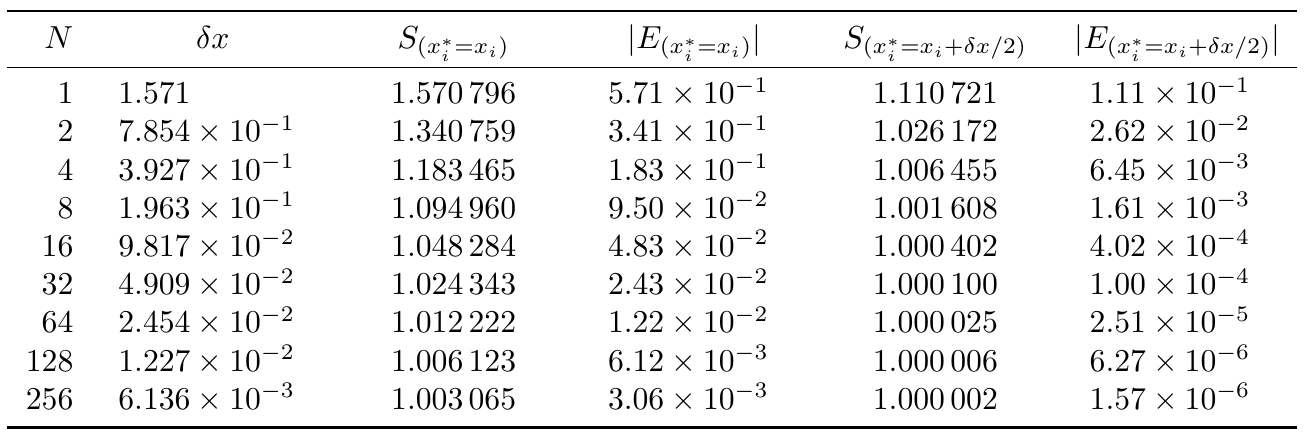
Let us do another verification, a numerical rather than a theoretical one. Let f(x) = sin(x), and let us calculate the integral of its derivative, df/dx = cos(x), from x = 0 to x = π/2, using successively refined Riemann sums. According to the fundamental theorem of calculus, we should obtain

$$ \int_0^{\pi/2} \frac{\mathrm{d}}{\mathrm{d}x}\left(\sin(x)\right) \, \mathrm{d}x \;=\; \int_0^{\pi/2} \cos(x) \, \mathrm{d}x \;=\; \sin(\pi/2) \;-\; \sin(0) \;=\; 1 $$

So, the Riemann sums must converge to the value 1. We will try Riemann sums of both the kind $x_i^* = x_i$ (left Riemann sums) and of the kind $x_i^* = x_i + \delta x/2$ (middle Riemann sums). The former are denoted as $S_{(x_i^*=x_i)}$ and the latter as $S_{(x_i^*=x_i+\delta x/2)}$ in the table of results below. The table records also the respective errors E (eq. ($\ref{Riemann sum}$)). We can notice that in the case $x_i^* = x_i$ every time δx is halved, E is also roughly halved. This means that E is proportional to δx. On the other hand, in the case $x_i^*=x_i+\delta x/2$ every time δx is halved, E becomes roughly 4 times smaller, which means that E is proportional to (δx)². Thus this numerical experiment confirms our theoretical expectations.

Here is some python code in case you want to try it yourself:

import numpy as np

# General function to compute a Riemann sum
def riemann_sum(f, a, b, n, method='left'):
    """
    Compute a Riemann sum for f on [a, b] with n intervals.
    method: 'left', 'right', or 'midpoint'
    """
    if n <= 0:
        raise ValueError("n must be positive")
    dx = (b - a) / n

    if method == 'left':
        xs = (a + i*dx for i in range(n))
    elif method == 'right':
        xs = (a + (i+1)*dx for i in range(n))
    elif method == 'midpoint':
        xs = (a + (i+0.5)*dx for i in range(n))
    else:
        raise ValueError("method must be 'left', 'right', or 'midpoint'")

    return dx * sum(f(x) for x in xs)


# Particular details for our chosen case
f = lambda x: np.sin(x)
dfdx = lambda x: np.cos(x)
xS = 0
xE = np.pi / 2
exact = f(xE) - f(xS)

# Header
print("Left & Midpoint Riemann sums of r(x)=cos(x) from x=0 to x=pi/2\n")
header = f"{'n':>8s}  {'dx':>12s}  {'Left Sum':>12s}  {'Err_L':>10s}  {'Mid Sum':>12s}  {'Err_M':>10s}"
print(header)
print("-" * len(header))

for l in range(9):
    n = 2**l
    dx = (xE - xS) / n
    lRS = riemann_sum(dfdx, xS, xE, n, 'left')
    mRS = riemann_sum(dfdx, xS, xE, n, 'midpoint')
    err_l = lRS - exact
    err_m = mRS - exact
    print(f"{n:8d}  {dx:12.3e}  {lRS:12.6f}  {err_l:10.2e}  {mRS:12.6f}  {err_m:10.2e}")

A different viewpoint

Up to this point we have placed our focus mostly on the differentiated function f(x), demonstrating the fundamental theorem of calculus through plots of f(x) vs. x such as the one repeated below for convenience. That plot demonstrates that the fundamental theorem of calculus essentially splits the change Δf = f(x_E) − f(x_S) into innumerable tiny changes δf_i, each of which is approximated as δf_i = r(x_i)δx_i where r(x) = df/dx is the derivative of f(x). (Of course, instead of r(x_i) we could use the derivative r($x_i^*$) at any other point $x_i^* \in [x_i, x_{i+1}]$, but $x_i^* = x_i$ is convenient for illustration purposes – the observations that follow apply for any $x_i^* \in [x_i, x_{i+1}]$). For any finite (non-zero) value of δx_i, an error will be involved, so that the accurate expression is δf_i = r(x_i)δx_i +ϵ_i. The plot below illustrates how δf_i is split into the two parts r(x_i)δx_i and ϵ_i. We can notice that the error ϵ_i is due to the curvature of f(x) within the interval [x_i, x_i+1]; had f(x) been completely straight within that interval, ϵ_i would have been zero and r(x_i)δx_i would capture the whole change δf_i = f(x_i+1) − f(x_i). However, as we noted earlier, for a smooth function f(x), as we consider smaller and smaller intervals δx_i, its behaviour within these smaller and smaller neighbourhoods is more and more linear; it locally behaves as a straight line. Thus, as we drive δx_i towards zero, ϵ_i as a percentage of δf_i becomes smaller and smaller, tending to 0% of δf_i , while r(x_i)δx_i becomes a larger and larger portion of δf_i, tending to 100% of it. We demonstrated this, both theoretically and by numerical experiments, for particular cases of functions such as f(x) = x², x³, and sin(x). Thus, in the limit δx_i → 0 the error goes away and we end up with the fundamental theorem of calculus,

$$ \begin{equation} \label{FTC again2} \int_{x_S}^{x_E} \frac{\mathrm{d}f}{\mathrm{d}x} \, \mathrm{d}x \;=\; \int_{x_S}^{x_E} r(x) \, \mathrm{d}x \;=\; f(x_E) - f(x_S) \end{equation} $$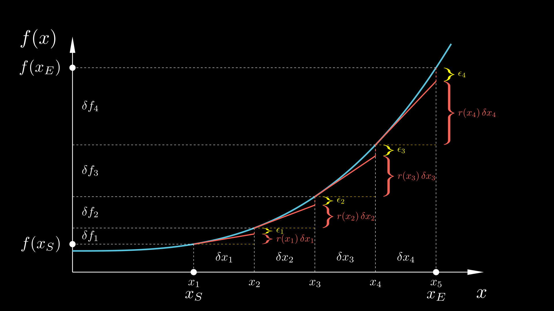

Now let us instead plot the derivative of f(x), r(x)=df/dx, and see what we make of this plot in relation to the fundamental theorem of calculus. The figure below contains essentially the same information as the figure above, only that it plots r(x) = df/dx instead of f(x). The red rectangles have width δx_i and height r(x_i), so that the area r(x_i)δx_i of each one is equal to the corresponding approximation of δf_i. Then, the yellow area above the rectangle and below the curve r(x) is the corresponding error ϵ_i.

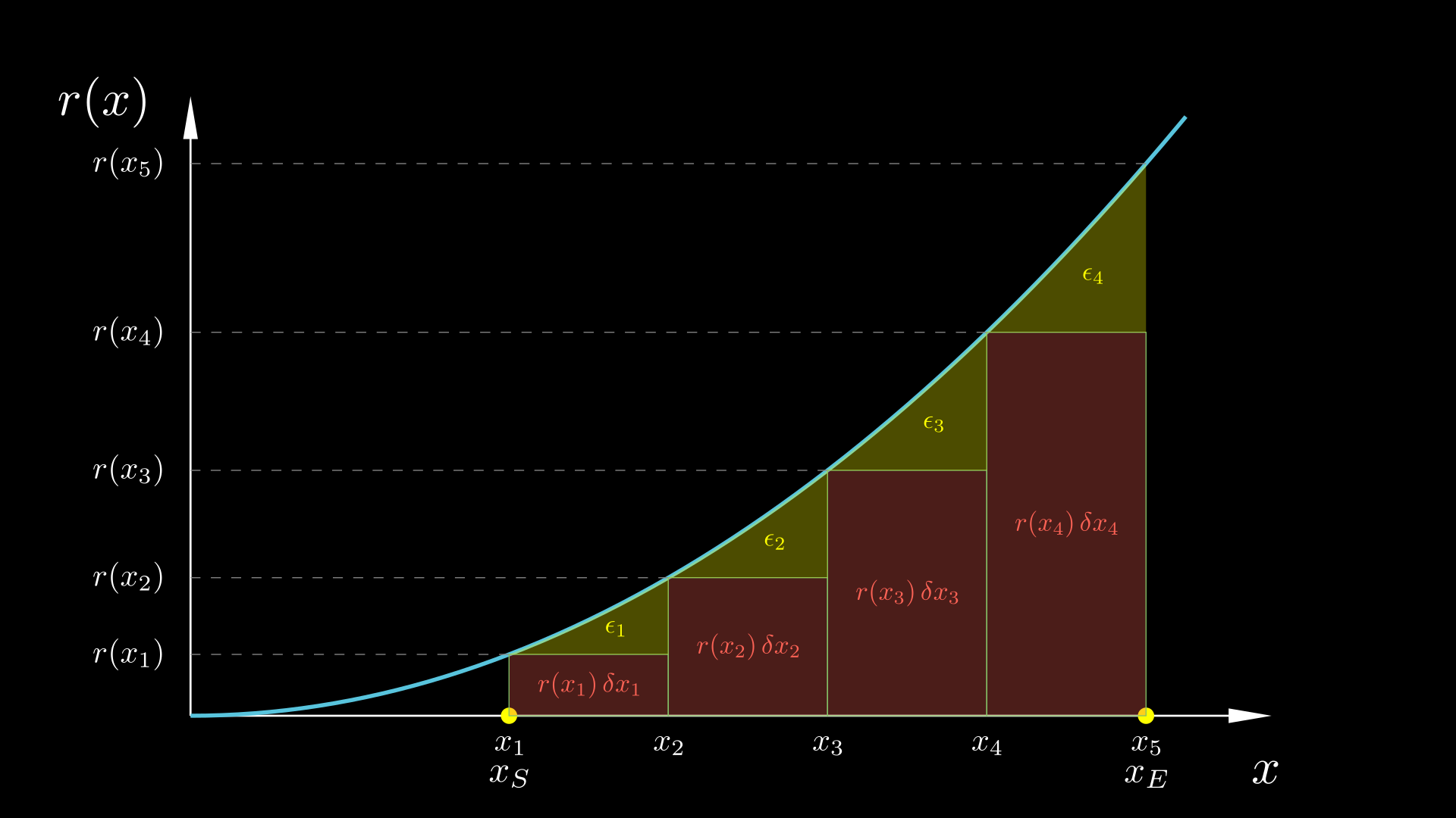
How do we know that the yellow area is the error? Well, we can be led to this conclusion by the following reasoning: if we refine the Riemann sums more and more by subdividing each of the original δx_i's into 2, 4, 8, etc. subintervals, then as the number of intervals goes to infinity we notice that the aggregate area of all rectangles, coloured in red, tends to become equal to the area bounded below by the x-axis, above by the curve r(x), and on the sides by x = x_S and x = x_E. At the same time, the left-over area below the r(x) curve that is outside of these rectangles, coloured in yellow, becomes smaller and smaller, tending to zero.

0:00

/0:27

1×

So, let us apply the fundamental theorem of calculus to a single coarse interval of those of the figure above:

$$ \begin{equation} \label{FTC single interval} f(x_{i+1}) - f(x_i) \;=\; \int_{x_i}^{x_{i+1}} r(x) \, \mathrm{d}x \end{equation} $$

According to what we just noted, the integral of the right-hand side, obtained as the limit of a left Riemann sum, is the area below the r(x) curve from x = x_i to x = x_i+1. Let us also write eq. ($\ref{df=dfdx.dx+e}$), with $x_i^* = x_i$, for that interval:

$$ \begin{equation} \label{df=r.dx+e single interval} f(x_{i+1}) - f(x_i) \;=\; r(x_i) \, \delta x_i \;+\; \epsilon_i \end{equation} $$

Comparing eqs. ($\ref{FTC single interval}$) and ($\ref{df=r.dx+e single interval}$), we see that their left-hand sides are the same, and therefore their right-hand sides must be equal, from which it follows that:

$$ \begin{equation} \label{ei} \epsilon_i \;=\; \int_{x_i}^{x_{i+1}} r(x) \, \mathrm{d}x \;-\; r(x_i) \, \delta x_i \end{equation} $$

Thus, indeed, ϵ_i is the difference between the area below r(x) from x = x_i to x = x_i+1 and the area of the rectangle i; it is the area painted yellow in the above figure.

Can we estimate ϵ_i? Yes, in fact we can, and it is instructive to do so. This is how we can proceed. Since r(x) is a function in its own right, if it is smooth, then it will also behave linearly (its plot will look like a straight line) in a small enough neighbourhood. Therefore, the yellow area that equals ϵ_i can be calculated as the area of a right triangle with base δx_i and height (r_i+1−r_i):

$$ \begin{align} \nonumber \epsilon_i \;&\approx\; \frac{1}{2} \, \delta x_i \, \left(r_{i+1} - r_i \right) \;\approx\; \frac{1}{2} \, \delta x_i \, \left. \frac{\mathrm{d}r}{\mathrm{d}x}\right|_{x_i} \delta x_i \\[0.2cm] \label{ei triangle} &=\; \frac{1}{2} \, \left. \frac{\mathrm{d}^2f}{\mathrm{d} x^2} \right|_{x_i} (\delta x_i)^2 \end{align} $$

where we have applied the concept of derivative to r(x) itself:

$$ \delta r_i \;\equiv\; r(x_{i+1}) - r(x_i) \;\approx\; \left. \frac{\mathrm{d}r}{\mathrm{d}x} \right|_{x_i} \delta x_i $$

And since r(x) is the derivative of f(x), the derivative of r(x) is the derivative of the derivative of f(x) (the rate of change of the rate of change of f(x) with respect to x), which is called the second derivative of f(x) and is denoted as d²f/dx².

---

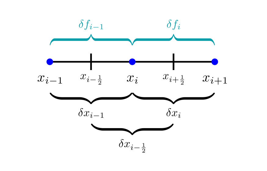
A quick detour: Why is the second derivative denoted this way? To see why, let us calculate it by using central differences that consider the first derivative at two neighbouring points and evaluate how fast it changes. Indeed, the second derivative is the rate of change of the first derivative. With reference to the figure below and the notation defined therein, the second derivative can therefore be approximated as:

$$ \left. \frac{\mathrm{d}^2f}{\mathrm{d}x^2} \right|_{x_i} \;\approx\; \frac{ \left. \dfrac{\mathrm{d}f}{\mathrm{d}x} \right|_{x_{i-\frac{1}{2}}} - \left. \dfrac{\mathrm{d}f}{\mathrm{d}x} \right|_{x_{i+\frac{1}{2}}} }{\delta x_{i-\frac{1}{2}}} \;\approx\; \frac{ \dfrac{\delta f_{i}}{\delta x_{i}} - \dfrac{\delta f_{i-1}}{\delta x_{i-1}} }{\delta x_{i-\frac{1}{2}}} $$

Note that there are two levels of approximation in the above expression: both the first and second derivatives are approximated via central differences.

If we choose the δx's equal then the above expression simplifies to:

$$ \begin{equation} \label{2nd derivative CD} \left. \frac{\mathrm{d}^2f}{\mathrm{d}x^2} \right|_{x_i} \;\approx\; \frac{\delta f_i - \delta f_{i-1}}{(\delta x)^2} \end{equation} $$

This approximation will become exact as δx → 0. The numerator of the above fraction is a difference of differences, so we could denote it as δ(δf) or δ²f. That is where the notation d²f/dx² for the 2^nd derivative comes from: the numerator is a difference of differences, while the denominator is the square of the interval size. So, we should interpret the denominator, dx², as (dx)², not d(x²).

---

Let us get back to the investigation of the errors involved in the Riemann summations. Equation ($\ref{ei triangle}$) gives us an estimate for an individual error ϵ_i of the approximation ($\ref{df=r.dx+e single interval}$). What about the total error, Ε =Σϵ_i, of the Riemann sum ($\ref{Riemann sum}$) though? For simplicity let us assume a uniform interval size δx. Then summing all the individual errors ($\ref{ei triangle}$) we get

$$ \begin{equation} \label{Sei LRS} \sum_{i=1}^N \epsilon_i \;=\; \frac{1}{2} \, N \, \overline{\frac{\mathrm{d}^2f}{\mathrm{d} x^2}} (\delta x_i)^2 \end{equation} $$

where the overlined second derivative is the average of the second derivatives at all points:

$$ \overline{\frac{\mathrm{d}^2f}{\mathrm{d} x^2}} \;\equiv\; \frac{1}{N} \sum_{i=1}^N \left. \frac{\mathrm{d}^2f}{\mathrm{d} x^2} \right|_{x_i} $$

The total number of points equals N = (x_E−x_S)/δx, which we can substitute in eq. ($\ref{Sei LRS}$) to arrive at

$$ \begin{equation} \label{Sei LRS 2} E \;=\; \sum_{i=1}^N \epsilon_i \;=\; \frac{x_E-x_S}{2} \, \overline{\frac{\mathrm{d}^2f}{\mathrm{d} x^2}} \delta x_i \end{equation} $$

This shows that while the individual errorsϵ_i are proportional to (δx)² and therefore decrease very rapidly with refinement (i.e. with diminishing δx), the overall error E decreases more slowly, proportionally to δx, because by making δx smaller we also increase the number of errors N that contribute to this sum (hence Zeno was not entirely wrong). This general theoretical result that, for $x_i^* = x_i$, E is proportional to δx, is in agreement with our corresponding earlier theoretical demonstration for the particular function f(x)=x² and with our numerical results for the function f(x)=sin(x).

Middle Riemann sums

The previous analysis concerned the case $x_i^* = x_i$. How about other cases? Well, most other cases are similar to the $x_i^* = x_i$ case; but the case $x_i^* = x_i + \delta x/2$ is somewhat special. The r(x) versus x diagram along with a middle Riemann sum is shown below, with the height of each rectangle i being equal to the value of r(x) at the midpoint of the interval, r(x_i + δx_i/2). What is the error ϵ_i now? We can see that it consists of two parts, painted in yellow and purple, respectively. The yellow part is how much the rectangle falls short of the area below the r(x) curve; but the purple part is how much the rectangle extends beyond the curve. Thus, the total error ϵ_i equals the yellow area minus the purple area.

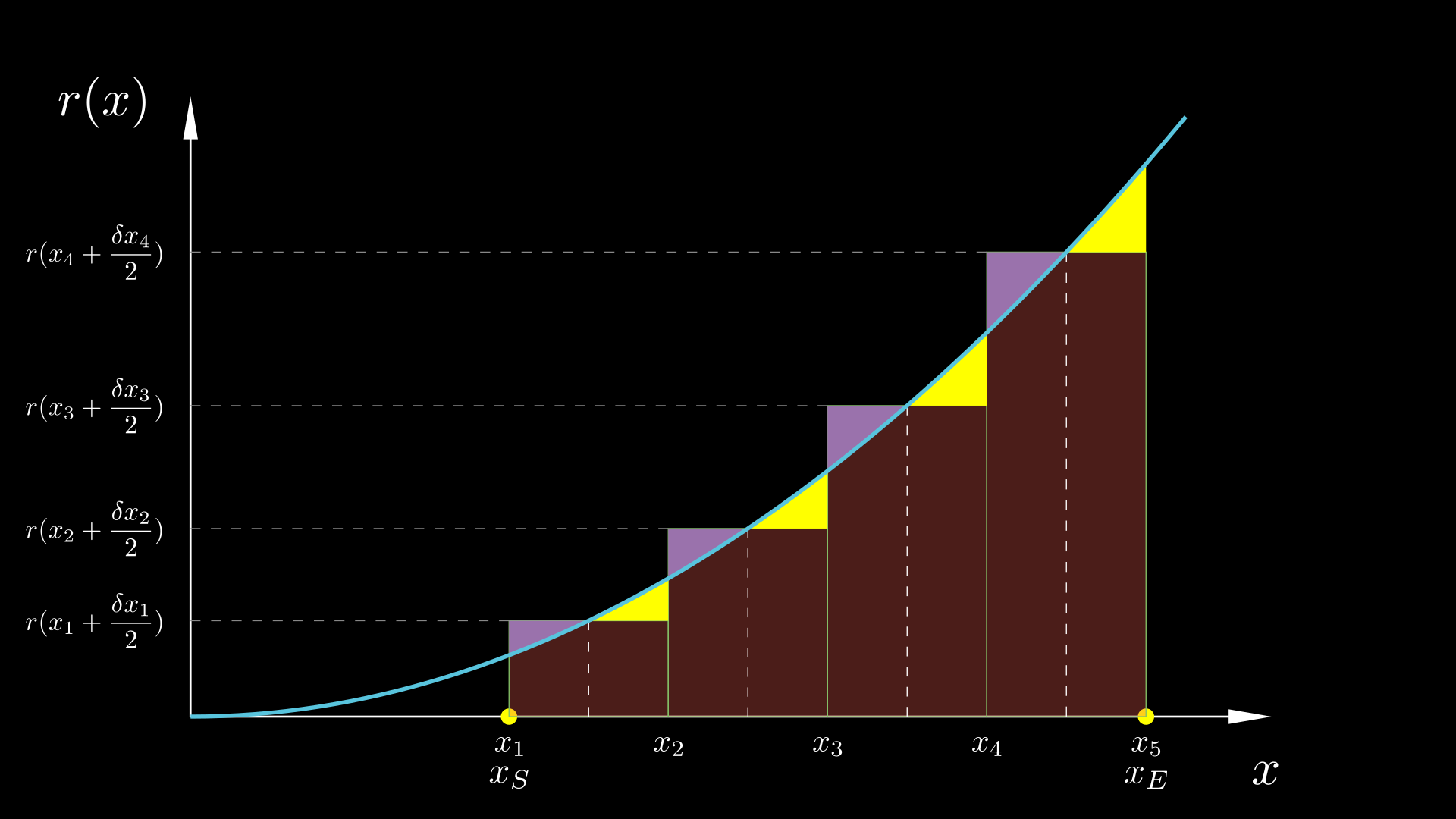
If we try to estimate this error in the same way as we did for the left Riemann sum, by assuming r(x) to be locally a straight line within the interval δx_i, then the yellow and purple triangles corresponding to that interval are obviously congruent and have the same area. Their corresponding contributions to the error, therefore, cancel each other out completely! The assumption of linear variation of r(x) within δx_i leads to the conclusion that ϵ_i is zero! This is why the Riemann sums with $x_i^* = x_i + \delta x/2$ have much smaller errors than the Riemann sums with $x_i^* = x_i$.

Of course, we do know that there is some non-zero error even for middle Riemann sums, as our theory and numerical experiments showed for particular cases. Actually, the condition that r(x) is a straight line does not obtain perfectly but only in the limit δx_i → 0. For any non-zero δx_i, r(x) will, in general, exhibit some curvature. The second derivative of r(x) is a measure of this curvature; the product

$$ \begin{equation} \label{r slope change} \left. \frac{\mathrm{d}}{\mathrm{d}x} \right|_{x_i} \!\! \left( \frac{\mathrm{d}r}{\mathrm{d}x} \right) \delta x_i \;=\; \left. \frac{\mathrm{d}^2 r}{\mathrm{d}x^2} \right|_{x_i} \delta x_i \end{equation} $$

is roughly how much the slope of r(x) changes between x = x_i and x = x_i + δx_i. So, for example, if r's second derivative is positive, then the slope dr/dx increases with x, and thus the vertical side of the yellow triangle will be larger than the vertical side of its purple brother. How much larger will it be? That depends not only on the slope difference between the hypotenuses of the two triangles, but also on their size, which is proportional to δx_i. In total then the vertical side of the yellow triangle will exceed the vertical side of the purple triangle by an amount proportional to the slope change ($\ref{r slope change}$) times the distance δx_i. Finally, we are not interested in the height difference per se but in the area difference; to find the area difference between the yellow and purple triangles we have to multiply their height difference by the length δx_i/2 of their horizontal side (the area of an orthogonal triangle is proportional to (height)×(width) therefore the difference in area is proportional to (difference in height)×(width)). Overall then δx_i appears three times as a factor, and the error is proportional to

$$ \begin{equation} \label{ei MRS} \epsilon_i \;\sim\; \left. \frac{\mathrm{d}^2 r}{\mathrm{d}x^2} \right|_{x_i} \! (\delta x_i)^3 \;=\; \left. \frac{\mathrm{d}^3 f}{\mathrm{d}x^3} \right|_{x_i} \! (\delta x_i)^3 \end{equation} $$

(as the second derivative of r(x) is the third derivative of f(x)). The total error Ε = Σϵ_i, just like in the $x_i^* = x_i$ case, will decrease more slowly, and in particular it will be proportional to (δx)³×(δx)⁻¹ = (δx)², because the total number N = (x_E−x_S)/δx of individual errors is proportional to (δx)⁻¹ (the smaller δx, the more rectangles and errors we have). This is in perfect agreement with our previous numerical experiments.

The derivative of the integral

Finally, let us turn to another aspect of the fundamental theorem of calculus. Up to now, we focused on the fact that r(x)dx = df and therefore the Riemann sum of all the products r(x)dx gives the total change of f(x) across our range. In other words, we viewed the fundamental theorem of calculus as expressing what happens when we integrate the derivative. Now let us examine the converse, what happens when we differentiate the integral.

Firstly we must convert the integral into a function, so that we can differentiate it. We can do this by fixing the lower bound of the integral at some value x₀ while allowing the upper bound to vary freely as the independent variable x. Let the integrated function be denoted as r(x) and the integral with the free upper boundary be denoted as f(x). These names are the same as we used before, and their choices already predispose you as to what the roles of these functions are, but let us forget about these roles for the moment, and view r(x) as a random function, and f(x) as defined by:

$$ \begin{equation} \label{integral as function} f(x) \;=\; \int_{x_0}^x r(x') \, \mathrm{d} x' \end{equation} $$

Note that, since the symbol x denotes the variable upper boundary of integration, we have to use a different symbol, x', for the integration variable. Indeed, during the integration process, for any given value of x, x' assumes a range of values different than x – in fact it assumes all values from x₀ to x.

Now let us try to calculate the derivative df/dx, i.e. the rate of change of f(x) with respect to x. This means that we want to calculate how fast the value of the integral changes if we nudge its upper boundary. To do so, we will turn to the fundamental definition of the derivative:

$$ \begin{align} \nonumber \frac{\mathrm{d}f}{\mathrm{d}x} \;&=\; \lim_{\delta x \rightarrow 0} \frac{f(x + \delta x) - f(x)}{\delta x} \\[0.2cm] \label{derivative of integral 0} &=\; \lim_{\delta x \rightarrow 0} \frac{\int_{x_0}^{x+\delta x} r(x') \mathrm{d}x' \;-\; \int_{x_0}^x r(x') \mathrm{d}x'}{\delta x} \end{align} $$

With reference to the following figure, the numerator in eq. ($\ref{derivative of integral 0}$) equals the area below the curve from x₀ to x+δx minus the area from x₀ to x. This difference is just the sum of the red and yellow areas:

$$ \begin{equation} \label{derivative of integral numerator} \int_{x_0}^{x+\delta x} r(x') \mathrm{d}x' \;-\; \int_{x_0}^x r(x') \mathrm{d}x' \;=\; r(x) \, \delta x \;+\; \epsilon \end{equation} $$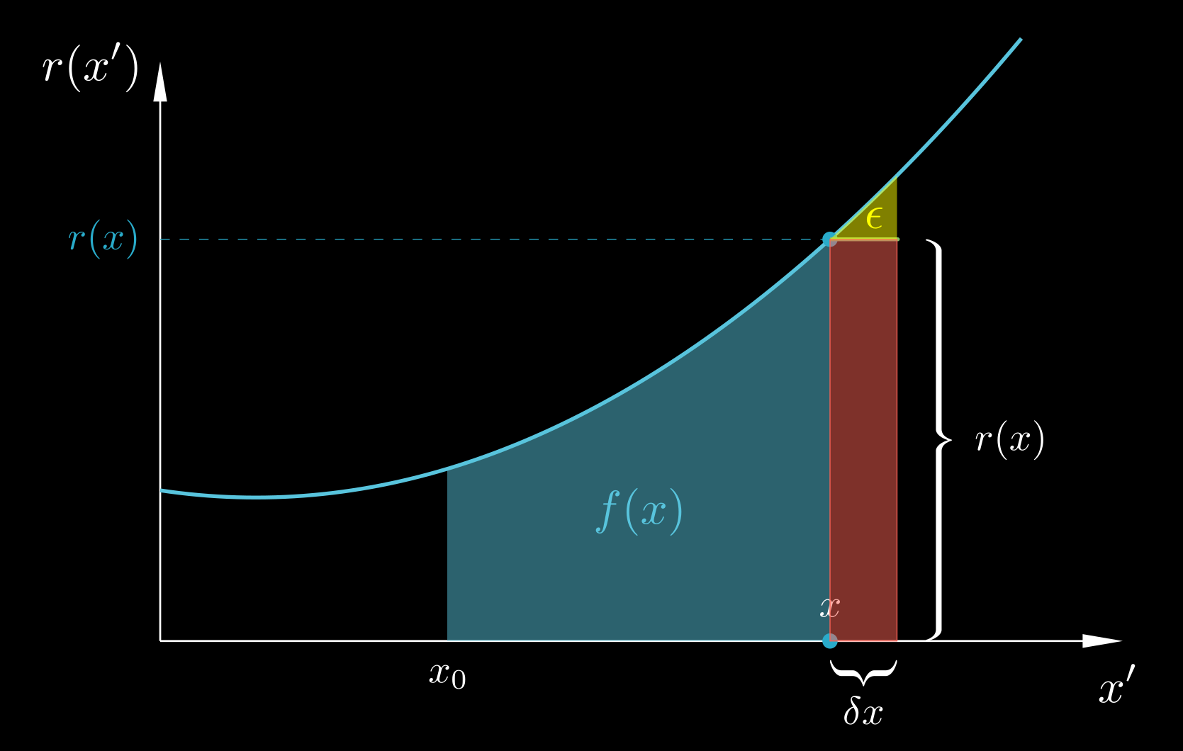

To estimate ϵ we can, like before, assume that since δx is small, r(x') is approximately linear within [x, x+δx] and thus the yellow area ϵ can be approximated as an orthogonal triangle of base δx and height δr = r(x+δx) − r(x) ≈ (dr/dx)δx, an approximation that becomes better and better as δx → 0. Therefore:

$$ \begin{equation} \label{derivative of integral e} \epsilon \;=\; \frac{1}{2} \frac{\mathrm{d}r}{\mathrm{d}x} \, (\delta x)^2 \end{equation} $$

(where the derivative is evaluated at the point x). Now let us substitute eqs. ($\ref{derivative of integral numerator}$) and ($\ref{derivative of integral e}$) into ($\ref{derivative of integral 0}$) to obtain:

$$ \begin{align} \nonumber \frac{\mathrm{d}f}{\mathrm{d}x} \;&=\; \lim_{\delta x \rightarrow 0} \frac{r(x) \, \delta x \;+\; \frac{1}{2} \frac{\mathrm{d}r}{\mathrm{d}x} \, (\delta x)^2}{\delta x} \\[0.3cm] \label{derivative of integral 1} &=\; \lim_{\delta x \rightarrow 0} \left( r(x) \;+\; \frac{1}{2} \frac{\mathrm{d}r}{\mathrm{d}x} \, \delta x \right) \;=\; r(x) \end{align} $$

We have therefore arrived at:

$$ \begin{equation} \label{derivative of integral} \frac{\mathrm{d}}{\mathrm{d}x} \int_{x_0}^x r(x') \, \mathrm{d} x' \;=\; r(x) \end{equation} $$

This result tells us that the rate of change of f(x) is equal to r(x), which actually makes sense: the larger the value of r(x), the faster the area f(x) will grow as we move x towards the right. In the limit δx → 0, the yellow error area ϵ becomes negligible compared to the red rectangle r(x)δx (proof: from eq. (44), ϵ/(r(x)δx) = (δx/2)(dr/dx)/r(x) → 0 as δx → 0), and therefore the whole change δf can be assumed to equal r(x)δx; hence the rate of increase of the area f(x) is δf/δx = (r(x)δx)/δx = r(x). Equation ($\ref{derivative of integral}$) is another expression of the fundamental theorem of calculus, showing that differentiation and integration are opposite operations, but instead of showing the effect of integrating the derivative as eq. ($\ref{FTC again2}$), it shows the effect of differentiating the integral.

Summary

At last, we have reached the end of this long post. We have looked at the fundamental theorem of calculus and the mathematical notions associated with it, including the notions of derivative, integral, and limit, from multiple angles, with the goal of acquiring an intuitive understanding of them. I hope that this goal has been met, and that you have enjoyed the journey! To summarise, the fundamental theorem of calculus tells us what happens when we (a) integrate a derivative and (b) differentiate an integral. The corresponding expressions are:

• Integration of a derivative:

$$ \begin{equation} \label{summary: integration of derivative} \int_{x_S}^{x_E} \frac{\mathrm{d}f}{\mathrm{d}x} \, \mathrm{d}x \;=\; f(x_E) \;-\; f(x_S) \end{equation} $$

• Differentiation of an integral:

$$ \begin{equation} \label{summary: differentiation of integral} \frac{\mathrm{d}}{\mathrm{d}x} \int_{x_0}^x f(x') \, \mathrm{d} x' \;=\; f(x) \end{equation} $$

Note that in eq. ($\ref{summary: differentiation of integral}$) we switched from denoting the integrated function as r(x), the notation used in ($\ref{derivative of integral}$), to the more generic name f(x), to highlight that both equations are applicable to general functions, without assuming any certain role to them.